Solving the Modified OU PDE and Calculate Mean Reversion rate

Calculating theta from the hazard rate curve:
We believe that the hazard rate follows the Ornstein-Uhlenbeck process
dh=α(θ-h)dt+σhdW
iven an initial term structure of hazard rate, we can find the value for θ by first calculating the closed form solution for the above pde and then eliminating the stochastic term from the solution.
We follow the integrating factor approch for finding the close form solution for the pde.
If we have a PDE of the form dX=F(t,X)dx+σXdW ,Initial Condition=X0
We can find the Integrating factor as
IF=exp(-∫sigma^tdw〖σdw+1/2∫sigma^tdw〖σ^2 dw〗〗)
Hence d(IF*X)=IF*F(t,X)dt
d(IF*X)/dt=IF*F(t,X)

h_t=h_0*exp⁡(-kt+σW_t )+α□(θ/k)*(1+exp(-k*t)
differentiating ht wrt time

∂h/∂t=h_0*exp⁡(-kt+σW_t )*(-k)+ α□(θ/k)*(exp(-k*t)*(-k)
∂h/∂t=(-k)(h_t- α□(θ/k))

θ=(∂h/∂t+k*h_t )/α
As we see our theta is dependent over the rate of change of h w.r.t to time and on the level of h as well. So our next task is to generate the different values ofθt, corresponding to the values of alpha and sigma.

Monte-Carlo simulation for dynamic hedging (Matlab)

The code below take the time steps as the input and display the difference between the delta hedge portfolio and the actual value for the call option and the standard error. The code also plots the histogram for that particular scenario(Y axis is number of occurrences in total and X axis is difference from the actual value) The histograms below compare the output of histogram for different values of rebalancing time (Denoted as n). The observation from this and the table for differences is that the delta hedge becomes more “efficient” as we increase the number of rebalancing steps. The x axis for n = 4 goes till +/- 20 while for n=250 the max deviation is reduced to +/- 2. Hence we can confidently say that delta hedging become more efficient as we increase the number of steps and it would eventually give zero difference with the actual value when n -> infinity.

Matlab Code:
%The function is checking the effectiveness of delta hedge
%by using Monte-carlo simulation Rebalancing time can be calculated
%Submitted By : Tanmay Dutta
%Simulation method for option Pricing
function [Difference,standard_error]= delta_hedgeH3_1(Rebalancing_time)
% Define the parameters for the option
K = 105;
T = 1;
n = 10000;
N = Rebalancing_time;
S0 = 100;
sigma = 0.1;
r = 0.05;
c = blsprice(S0,K,r,T,sigma,0.0);
% Define what are needed for calculations
Z = randn(n,N);
S = zeros(n,N);
t_increment = T/Rebalancing_time;
timeToMaturity = T-t_increment;
S(:,1)=S0*exp((r-0.5*sigma*sigma)*T/N+sigma*Z(:,1)*sqrt(T/N));
Delta_prev = calculate_callDelta(S(:,1),K,r,sigma,timeToMaturity);
Stock_Position_P = Delta_prev.*S(:,1);
Bond_Position = c-Stock_Position_P;
for i = 2:N
Bond_Position = Bond_Position*exp(r*t_increment); %Bond has grown to this value
S(:,i)=S(:,(i-1)).*exp((r-0.5*sigma*sigma)*T/N+sigma*Z(:,i)*sqrt(T/N)); % New stock process
timeToMaturity = timeToMaturity-t_increment; % time has passed
if i Delta_new = calculate_callDelta(S(:,i),K,r,sigma,timeToMaturity);
Stock_adjustment = (Delta_new-Delta_prev).*S(:,i);
Bond_Position = Bond_Position - Stock_adjustment;
Stock_Position_P = Delta_new.*S(:,i);
else
Stock_Position_P=Delta_new.*S(:,N);
end
Delta_prev = Delta_new;
end
Final_value = Stock_Position_P+Bond_Position;
%hist(Final_value,500);
call = max(S(:,N)-K,0);
%figure;hist(call,500);
Difference = Final_value-call; %-max(S(:,N)-K,0);
hist(Difference,500);
title(strcat('Difference for n =',num2str(Rebalancing_time)));
standard_error=std(Difference)/sqrt(n);
Difference = mean(Difference);
end
function delta = calculate_callDelta(S0,K,R,Sigma,T)
delta = (log(S0/K)+(R+0.5*Sigma^2)*T)/(Sigma*sqrt(T));
delta = normcdf(delta);
end

Basic Mathematics Problems

These problems are some of very famous and chosen by me for my own interview preparations.

(Just for someone interested and ignorant.. the best site for detailed solutions would be wolfram-alpha)

First Problem

Differentiate x^x

Answer: We do it by chain rule assume it as fx^gx so we apply chain rule on this function [d fx^gx/d(fx)]x d(fx)/dx + [d fx^gx/dgx ]x d(gx)/dx

hence the answer would be (1+log(x)) x^x

^{(Just noticed another way, this one is not brute force but rather smart way)}

^{y =} x^x

^{take log}

^{log y = xlogx}

^{now differentiate}

^{dy/y = (logx + x/x)}

^{=> dy = y(logx +1)}

^{same as above ( Maths is consistent when correct :) )}

^{Second problem}

Integrate cos²(x) and cos³(x).

cos(2A) = 2cos²(x)-1

=> cos²(x) = [1+cos(2A)]/2

rest is pretty simple

for cos³(x) write it as cos(x)cos²(x) now write squared terms in form of sin and then put sin(x) as y then cos(x)dx would be dy so we will have Integral(1-Y²)dy

rest is simple for this one as well.

Third problem

What is 1.06 raised to the power 10.5

let y = 1.06^10.5

then ln y = 10.5X ln(1.06)

ln(1+x) when x tends to zero is equal to x

hence ln(1.06) can be approximated to 0.06

hence

lny = 0.63

hence y = exp(0.63) which could be approximated around 1.8

(this was the first method that came to my mind)

Brownian motion simulations

Matab code for generating Arithmetic Brownian motion

%This code is written by Tanmay Dutta

function val=ABM_simulation(time,step)

delta=(time/step)^0.5; %This is how we define the delta in BM

p = 0.5; % probability of random walk up or down

val=zeros(1,step);

u=zeros(1,step);

for i=1:numel(u)

u(i)=rand;

%%%%% NOTE ' ' NEAR GREATER AND LESS SIGNS. IF

%% YOU WANT TO REUSE THE CODE REMOVE ' ' IN NEXT LINE

val=delta*(p'<'u)-delta*(p'>'u);

end

for k=2:numel(val)

val(k)=val(k)+val(k-1);

end

val(1)=0.00 % Because B(0) =0 always

end

One simulation result for my code :

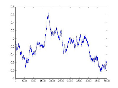
(Simulation on T=[0-1] and step = 5000)

(Note that the level goes below zero too, hence it can not be used for stock modeling and we need geometric Brownian motion with drift for that case )

Simulation of different random variables

To simulate a random variable of CDF (note its CDF not PDF) the easiest way is
x = F(inverse) [rand()]
rand() = uniform random variable(matlab and excel has standard functions for this)
Of course this works only when we have some closed form expression for CDF..
Hence will not work for distributions like Gaussian etc.
I will be updating this page for simulating different distributions using matlab

LU factorization for a tridigonal matrix in VBA

Option Base 1
Sub Tridiagonal_solver()
A_Mat = Range("A1:E5")
coeff = Range("H1:H5")
Dim n As Integer
n = UBound(A_Mat, 1)
Dim l_mat() As Double, u_mat() As Double, alpha As Double, beta As Double, y_array() As Double
ReDim y_array(n) As Double
ReDim l_mat(n, n) As Double
ReDim u_mat(n, n) As Double
For i = 1 To n
For j = i To n
l_mat(i, j) = 0
u_mat(i, j) = 0
Next j, i

For i = 1 To n
If (i = 1) Then
u_mat(i, i) = A_Mat(i, i)
End If
l_mat(i, i) = 1

If (i > 1) Then
u_mat(i, i - 1) = A_Mat(i, i - 1)
l_mat(i, i - 1) = A_Mat(i, i - 1) / u_mat(i - 1, i - 1)
u_mat(i, i) = A_Mat(i, i) - l_mat(i, i - 1) * A_Mat(i - 1, i)
End If
Next i
For i = 1 To n
If (i = 1) Then
y_array(i) = coeff(i)
End If

Next i
Range("A8:E12") = l_mat
Range("H8:L12") = u_mat

End Sub

C++ simulation for a puzzle

Sometimes we can find the answers by simulations easier than by logic. (In this case logic is also pretty easy )
The problem : On what day Sat/Sun(For that matters any combination ) will 1st of january fall mostly( Again for that matter any date )
// Purpose : The code try to simulate all the years till 2401 and find which day is on 31st december each year
//Logic:
// Because of the leap year rule we have exacly (400*365+100-3) day and its divisible by 7 completely hence we just
// need to check till 400 years
// Author: Tanmay Dutta
#include
#define start 2002
#define end 2401
using namespace std;
int main()
{
int year,day,count[7];
bool isleap,iscentury;
isleap= false;
iscentury = false;
day=0;
// initializing count to zero
for(int i =0;i<7; i++)
count[i]=0;
enum weekdays{ mon,tue,wed,thr,fri,sat,sun}; // starts with monday = 0
// We know that on 2010 31st dec was on friday
count[day]=1;
for(year = start; year<=end; year++)
{
// check for leap year
if(year%4 ==0)
isleap=true;
// leap year rule does not apply to years with last two digits as 100
if(year%100==0)
isleap = false;
// this rule has an exception at 400 again
if(year%400==0)
isleap=true;
if(isleap)
day=day+2;
else
day=day+1;
if(day==7)
day = 0;
if(day==8)
day=1;
isleap = false;
count[day]+=1;
}
cout<<"Mon"<<'\t'<<"Tue"<<'\t'<<"Wed"<<'\t'<<"Thr"<<'\t'<<"Fri"<<'\t'<<"Sat"<<'\t'<<"Sun"<<'\n';
for(int i =0;i<7; i++)
cout< cout<<'\n';
system("PAUSE");

}